summarize_at(my_data,
.vars = vars(starts_with("IND")),
.funs = list(sum, mean))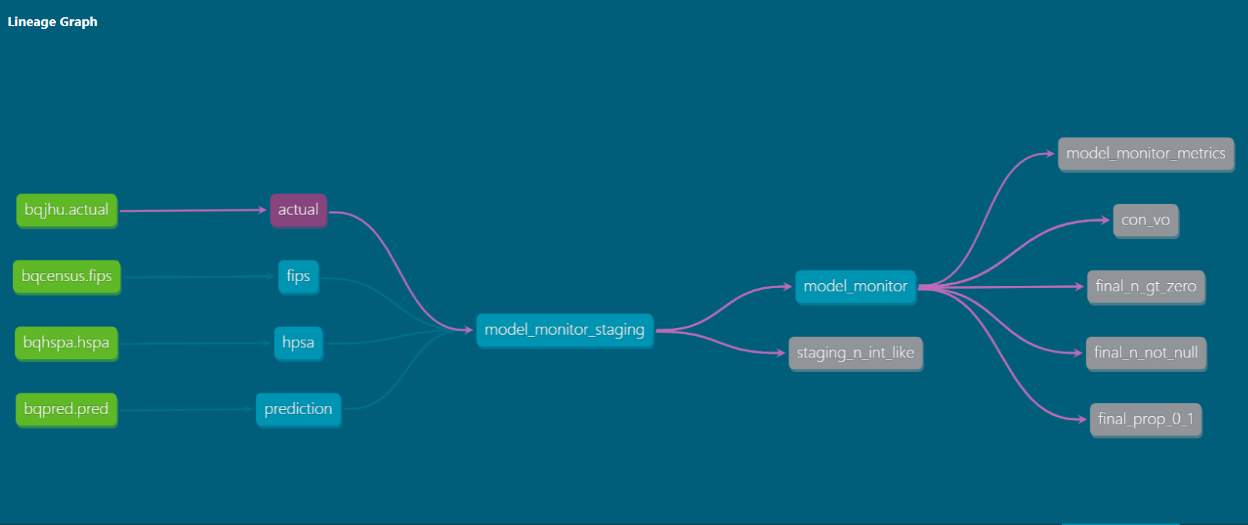 In my post Column Names as Contracts, I explore how using controlled vocabularies to name fields in a data table can create performance contracts between data producers and data consumers1. In short, I argue that field names can encode metadata2 and illustrate with R and python how these names can be used to improve data documentation, wrangling, and validation.
However, demonstrations with R and python are biased towards the needs of data consumers. These popular data analysis tools provide handy, high-level interfaces for programmatically operating on columns. For example, dplyr’s select helpers make it easy to quickly manipulate all columns whose names match given patterns. For example, suppose I know that all variables beginning with IND_ are binary and non-null so I may sum them to get a count or average them to get a valid proportion. I can succinctly write:
In contrast, SQL remains a mainstay for data producers – both for use in traditional relational databases and SQL interfaces for modern large-scale data processing engines like Spark. As a very high-level and declarative language, SQL variants generally don’t offer a control flow (e.g. for loops, if statements) or programmatic control which would allow for column operations that are similar to the one shown above. That is, one might have to manually write:
select
  mean(ind_a),
  mean(ind_b),
  sum(ind_a),
  sum(ind_b)
from my_data
But that is tedious, static (would not automatically adapt to the addition of more indicator variables), and error-prone (easy to miss or mistype a variable).
Although SQL itself is relatively inflexible, recent tools have added a layer of “programmability” on top of SQL which affords far more flexibility and customization. In this post, I’ll demonstrate how one such tool, dbt, can help data producers consistently apply controlled vocabularies when defining, manipulating, and testing tables for analytical users.
(In fact, after writing this post, I’ve also begun experimenting with a dbt package, dbt_dplyr that brings dplyr’s select-helper semantics to SQL.)
A brief intro to dbt
dbt (Data Build Tool) “applies the principles of software engineering to analytics code”. Specifically, it encourages data producers to write modular, atomic SQL SELECT statements in separate files (as opposed to the use of CTEs or subqueries) from which dbt derives a DAG and orchestrates the execution on your database of choice3. Further, it enables the ability to write more programmatic (with control flow) SQL templates with Jinja2 which dbt compiles to standard SQL files before executing.
For the purposes of implementing a controlled vocabulary, key advantages of this approach include:
- Templating with
ifstatements andforloops - Dynamic insertion of local variables4
- Automated testing of each modular SQL unit
- Code sharing with tests and macros exportable in a package framework
Additional slick (but tangential for this post) dbt features include:
- The ability to switch between dev and production schemas
- Easy toggling between views, tables, and inserts for the same base logic
- Automatic generation of a static website documenting data lineage, metadata, and test results (the featured image above is a screenshot from the created website)
- Orchestration of SQL statements in the DAG
- Hooks for rote database management tasks like adding indices and keys or granting access
For a general overview to dbt, check out the introductory tutorial on their website, the dbt101 presentation from their recent Coalesce conference5, or the interview with one of their founders on the Data Engineering Today podcast.
In this post, I’ll demonstrate how three features of dbt can support the use of controlled vocabulary column naming by:
- Creating variable names that adhere to conventions with Jinja templating
- Operating on subgroups of columns created by custom macros to enforce contracts
- Validating subgroups of columns to ensure adherence to contracts with custom tests
Scenario: COVID Forecast Model Monitoring
The full example code for this project is available on GitHub.
To illustrate these concepts, imagine we are tasked with monitoring the performance of a county-level COVID forecasting model using data similar to datasets available through Google BigQuery public dataset program. We might want to continually log forecasted versus actual observations to ask questions like:
- Does the forecast perform well?
- How far in advance does the forecast become reliable?
- How does performance vary across counties?
- Is the performance acceptable in particularly sensitive counties, such as those with known health professional shortages?
Before we go further, a few caveats:
- I am not a COVID expert nor do I pretend to be. This is not a post about how one should monitor a COVID model. This is just an understandable, hypothetical example with data in a publicly available database6
- I do not attempt to demonstrate the best way to evaluate a forecasting model or a holistic approach to model monitoring. Again, this is just a hypothetical motivation to illustrate data management techniques
- This may seem like significant over-engineering for the problem at hand. Once again, this is just an example
Now, back to work.
Controlled Vocabulary
To operationalize this analytical goal, we might start out by defining our controlled vocabulary with relevant concepts and contracts.
Units of measurement:
ID: Unique identifier of entity with no other semantic meaning- Non-null
N: Count- Integer
- Non-null
DT: Date- Date format
IND: Binary indicator- Values of 0 or 1
- Non-null
PROP: Proportion- Numeric
- Bounded between 0 and 1
PCT: Percent- Numeric
- Unlike
PROP, not bounded (e.g. think “percent error”)
CD: System-generated character- Non-null
NM: Human-readable name
Units of observation:
COUNTY: US CountySTATE: US StateCASE: Realized case (in practice, we would give this a more specific definition. What defines a case? What sort of confirmation is required? Is the event recorded on the date or realization or the date of reporting?)HOSP: Realized hospitalization (same note as above)DEATH: Realized death (same note as above)
Descriptors:
ACTL: Actual observed valuePRED: Predicted valueHPSA: Health Professional Shortage Area (county-level measure)
Data Sources and Flow
Our goal is to end up with a model_monitor table with one record per observation date and county (same as the actual table). Using the grammar above, we may define the variables we intend to include in our final table:
CD_(COUNTY|STATE): Unique county/state identifier (from Census Bureau FIPS codes)NM_(COUNTY|STATE): Human-readable county/state names-DT_COUNTY: The date a county’s values are observedN_(CASE|HOSP|DEATH)_(ACTL|PRED)_(07|14|21|28): The actual or predicted number of cases, hospitalizations, or deaths (and, for predictions only, the value of these predictions at 7, 14, 21, and 28 days prior to the day being forecasted)IND_COUNTY_HPSA: Indicator of whether county is considered a shortage areaPROP_COUNTY_HPSA: Proportion of population that is underserved in a designated shortage area
We will source these fields from four tables:
actualtable- sourced from
bigquery-public-data.covid19_jhu_csse.summary - one record per
observation datexcounty - fields for county code, observation date, realized number of cases and deaths
- sourced from
predictiontable- sourced from
bigquery-public-data.covid19_public_forecasts.county_28d_historical - one record per
date prediction was madexdata being predictedxcounty(initially) - fields for county code, observation date, prediction date, predicted number of cases and deaths
- we transform to one record per
observation datexcountywith observations at different time lags represented as separate fields
- sourced from
hpsatable- sourced from
bigquery-public-data.sdoh_hrsa_shortage_areas.hpsa_primary_care - (after some wrangling on our end) one record per
countyfor counties identified as having a shortage - fields for the county code, date of designation, proportion of county under-served
- sourced from
fipstable7- sourced from
bigquery-public-data.census_utility.fips_codes_all - (after some wrangling) one record per
countyfor each county in the 50 US states - fields for FIPS code (Census Bureau county identifiers), state name, county name
- sourced from
For a conceptual mental map, once all the wrangling and cleaning is done for each of the tables above, we might have psuedocode for the final table that looks something like this.
select *
from
  actual
    left join
  predictions using (cd_county, dt_county)
    left join
  hpsa using (cd_county)
    left join
  fips using (cd_county)
But as we’re about to see, dbt allows us to get a bit more complex and elegant.
Variable Creation with Jinja Templating
dbt makes it easy to create typo-free variable names that adhere to our controlled vocabulary by using the Jinja templating language.8 Jinja brings traditional control-flow elements like conditional statements and loops to make SQL more programmatic. When dbt is executed with dbt run, it first renders this Jinja to standard SQL before sending the query to the database.
Templates, and specifically loops, help write more concise and proof-readable SQL code when deriving a large number of variables with similar logic. For example, below we collapse the raw prediction data (which is represented as one record for each county x each day being prediction x each day a prediction was made) to one record for each county and each day being predicted with different columns containing the numeric value of each prediction of cases, hospitalizations, and deaths at lags (defined in the dbt_project.yml configuration file) of 7, 14, 21, and 28 days prior to the date being predicted.
Ordinarily, deriving these 12 variables (3 measures x 4 lags) would pose significant room for typos in either the code or the variable names, but in this script, the Jinja template of n_case_pred_{{l}} ensures consistency.
{{
    config(
        materialized='incremental',
        unique_key= 'id'
    )
}}

select
  county_fips_code || ' ' || forecast_date as id,
  county_fips_code as cd_county,
  forecast_date as dt_county,
  {% for l in var('lags') %}
    max(if(date_diff(prediction_date, forecast_date, day) = {{l}},
         round(100*new_confirmed, 0), null)) as n_case_pred_{{l}},
    max(if(date_diff(prediction_date, forecast_date, day) = {{l}},
         round(100*hospitalized_patients, 0), null)) as n_hosp_pred_{{l}},
    max(if(date_diff(prediction_date, forecast_date, day) = {{l}},
         round(100*new_deaths, 0), null)) as n_death_pred_{{l}}
  {% if not loop.last %},{% endif %}
  {% endfor %}
from {{ source('bqpred', 'pred') }}
where
  cast(left(county_fips_code, 2) as int64) between 1 and 56 and
  forecast_date <= current_date()
  {% if is_incremental() %}
  and forecast_date >= (
    select dateadd(day, -7, max(dt_county)) from {{this}}
  )
  {% endif %}
group by 1,2,3
This script renders to the following:
select
  county_fips_code || ' ' || forecast_date as id,
  county_fips_code as cd_county,
  forecast_date as dt_county,

    max(if(date_diff(prediction_date, forecast_date, day) = 07,
         round(100*new_confirmed, 0), null)) as n_case_pred_07,
    max(if(date_diff(prediction_date, forecast_date, day) = 07,
         round(100*hospitalized_patients, 0), null)) as n_hosp_pred_07,
    max(if(date_diff(prediction_date, forecast_date, day) = 07,
         round(100*new_deaths, 0), null)) as n_death_pred_07
  ,

    max(if(date_diff(prediction_date, forecast_date, day) = 14,
         round(100*new_confirmed, 0), null)) as n_case_pred_14,
    max(if(date_diff(prediction_date, forecast_date, day) = 14,
         round(100*hospitalized_patients, 0), null)) as n_hosp_pred_14,
    max(if(date_diff(prediction_date, forecast_date, day) = 14,
         round(100*new_deaths, 0), null)) as n_death_pred_14
  ,

    max(if(date_diff(prediction_date, forecast_date, day) = 21,
         round(100*new_confirmed, 0), null)) as n_case_pred_21,
    max(if(date_diff(prediction_date, forecast_date, day) = 21,
         round(100*hospitalized_patients, 0), null)) as n_hosp_pred_21,
    max(if(date_diff(prediction_date, forecast_date, day) = 21,
         round(100*new_deaths, 0), null)) as n_death_pred_21
  ,

    max(if(date_diff(prediction_date, forecast_date, day) = 28,
         round(100*new_confirmed, 0), null)) as n_case_pred_28,
    max(if(date_diff(prediction_date, forecast_date, day) = 28,
         round(100*hospitalized_patients, 0), null)) as n_hosp_pred_28,
    max(if(date_diff(prediction_date, forecast_date, day) = 28,
         round(100*new_deaths, 0), null)) as n_death_pred_28


from `bigquery-public-data`.`covid19_public_forecasts`.`county_28d_historical`
where
  cast(left(county_fips_code, 2) as int64) between 1 and 56 and
  forecast_date <= current_date()

group by 1,2,3
This script and the other three that derive our base tables (actual, prediction, fips, and hpsa) can be found in the models directory of the repo. After they are individually created, they are combined into the model_monitor_staging table in the relatively uninteresting script:
{{
    config(
        materialized='incremental',
        unique_key='id'
    )
}}

select
  actual.*,
  prediction.* except (cd_county, dt_county, id),
  fips.* except (cd_county),
  hspa.* except (cd_county)
from
  {{ ref('actual') }} as actual
  inner join
  {{ ref('prediction') }} as prediction
  using (dt_county, cd_county)
  left join
  {{ ref('fips') }} as fips
  using (cd_county)
  left join
  {{ ref('hpsa') }} as hspa
  using (cd_county)
{% if is_incremental() %}
where dt_county >= (
  select dateadd(day, -7, max(dt_county)) from {{this}}
  )
{% endif %}
Variable Manipulation with Regex Macros
Of course, it’s not enough to adhere to controlled vocabulary naming. If the actual contracts implied in those names are not upheld, the process is meaningless (or, worse, dangerous). When preparing our final table, we want to explicitly enforce as many of the vocabulary’s promises to be met as possible. This means, for example, ensuring all variables prefixed with n are really integers, dt are truly dates (and not just similarly formatted strings), and ind variables are actually never-null.
This time, we again use Jinja templating along with another dbt feature: custom macros. The final script in our pipeline (model_monitor) uses custom macros get_column_names() to determine all of the column names in the staging table and get_matches() to subset this list for variable names which match regular expressions corresponding to different prefixes.
Then, we iterate over each of these lists to apply certain treatments to each set of columns such as casting cols_n and cols_dt variables to int64 and date respectively, rounding cols_prop variables to three decimal places, and coalescing cols_ind variables to be 0 if null.9
{{
    config(
        materialized='incremental',
        unique_key='id',
        partition_by={
          "field": "dt_county",
          "data_type": "date",
          "granularity": "month"
        }
    )
}}

{% set cols = get_column_names( ref('model_monitor_staging') ) %}
{% set cols_n = get_matches(cols, '^n_.*') %}
{% set cols_dt = get_matches(cols, '^dt_.*') %}
{% set cols_prop = get_matches(cols, '^prop_.*') %}
{% set cols_ind = get_matches(cols, '^ind_.*') %}
{% set cols_oth = cols
   | reject('in', cols_n)
   | reject('in', cols_dt)
   | reject('in', cols_prop)
   | reject('in', cols_ind) %}

select

   {%- for c in cols_oth %}
   {{c}},
   {% endfor -%}
   {%- for c in cols_n %}
     cast({{c}} as int64) as {{c}},
   {% endfor %}
   {%- for c in cols_dt %}
     date({{c}}) as {{c}},
   {% endfor -%}
   {%- for c in cols_prop %}
     round({{c}}, 3) as {{c}},
   {% endfor -%}
   {%- for c in cols_ind %}
     coalesce({{c}}, 0) as {{c}}
     {% if not loop.last %},{% endif %}
   {% endfor -%}

from {{ ref('model_monitor_staging') }}

{% if is_incremental() %}
where dt_county >= (
  select dateadd(day, -7, max(dt_county)) from {{this}}
  )
{% endif %}
Note how abstract this query template is. In fact, it completely avoids referencing specific variables in our table.10 If we should decide to go back and add more fields (for example, actual and predicted recoveries) into our upstream models, they will receive the correct post-processing and validation as long as they are named appropriately.
For a peak under the hood, here’s how those two macros work.
First, get_column_names() simply queries the databases’ built in INFORMATION_SCHEMA11 to collect all column names of a given table. In the case of the model_monitor.sql script, the table provided is the staging table (model_monitor_staging) which was made in the previous step.
{% macro get_column_names(relation) %}

{% set relation_query %}
select column_name
FROM {{relation.database}}.{{relation.schema}}.INFORMATION_SCHEMA.COLUMNS
WHERE table_name = '{{relation.identifier}}';
{% endset %}

{% set results = run_query(relation_query) %}

{% if execute %}
{# Return the first column #}
{% set results_list = results.columns[0].values() %}
{% else %}
{% set results_list = [] %}
{% endif %}

{{ return(results_list) }}

{% endmacro %}
Next, the get_matches() macro simply iterates through a list of characters (such as the column names obtained in the previous step) and appends only those that match our regex to the final list that is returned.12 13 (Thanks to David Sanchez on the dbt Slack community for helping me figure out how to call the re library from within Jinja.)
{% macro get_matches(input_list, regex) %}

{% set results_list = [] %}
{% for l in input_list %}
    {% if modules.re.match(regex, l, modules.re.IGNORECASE) %}
        {{ results_list.append(l) or "" }}
    {% endif %}
{% endfor %}

{{ return(results_list) }}

{% endmacro %}
These macros live in the macros/ directory of the repository.
Data Validation with Custom Tests
Of course, not every contract can be made by force without risk of corrupting data. For any that we cannot enforce in their creation, we must rigorously test.
dbt’s testing framework allows for testing any data model in the project – not just the final table. This is very useful to intercept errors as soon as they happen instead of trying to backtrack from bad output many steps later. Some tests are built-in but others can be custom written as SQL SELECT statements.
Built-in tests for properties of individual columns include unique, not_null, and relationship14. These can be implemented in the schema.yml configuration file under the tests key-value pair for each relevant column, and can sometimes be shared across models with the YAML & and * (as shown below with the same basetest checks being applied to the actual and prediction data models) which allows for naming and repeating blocks (think copy-paste). However, even with a relatively small number of tests and columns, its cumbersome and easy to overlook a column.
version: 2

sources:
  - name: bqhspa
    description: HRSA designated shortage areas
    database: bigquery-public-data
    schema: sdoh_hrsa_shortage_areas
    tables:
      - name: hpsa
        identifier: hpsa_primary_care
  - name: bqcensus
    description: >
      Census Bureau mapping of FIPS codes to county and state names
    database: bigquery-public-data
    schema: census_utility
    tables:
      - name: fips
        identifier: fips_codes_all
  - name: bqjhu
    description: >
      Daily COVID case and death statistics by county
      from the Johns Hopkins University CSSE
    database: bigquery-public-data
    schema: covid19_jhu_csse
    tables:
      - name: actual
        identifier: summary
  - name: bqpred
    description: Forecasted case and death statistics
    database: bigquery-public-data
    schema: covid19_public_forecasts
    tables:
      - name: pred
        identifier: county_28d_historical

models:
  - name: actual
    description: >
      Actual COVID cases and deaths by county
    columns: &basetest
      - name: id
        tests:
          - unique
          - not_null
      - name: cd_county
        tests:
          - relationships:
              to: ref('fips')
              field: cd_county
  - name: prediction
    description: >
      Predicted COVID cases and deaths by county
    columns: *basetest
  - name: hpsa
    description: >
      Counties designated as healthcare shortage areas
    columns:
      - name: cd_county
        tests:
          - unique
          - not_null
          - relationships:
              to: ref('fips')
              field: cd_county
  - name: fips
    description: >
      Mapping of county and state names from FIPS codes
    columns:
      - name: cd_county
        tests:
          - unique
          - not_null
  - name: model_monitor_staging
    description: >
      Staging table to combine different data sources
  - name: model_monitor
    description: >
      Final model monitoring table with one row per county x observed day
    columns:
      - name: id
        test:
        - unique
        - not_null
      - name: ind_county_hpsa
        tests:
        - not_null
        - accepted_values:
            values: [0,1]
            quote: false
      - name: prop_county_hpsa
        tests:
          - dbt_utils.not_null_where:
              where: "ind_county_hpsa = 1"
Instead, developers may also define custom tests as SQL SELECT statements which returns only records that fail the test. Like data models, tests may also use Jinja and macros. This allows us to abstract some of our data validation tests to target all variables with a specific naming convention (and, thus, performance contract) at any arbitrary point in the pipeline.
For example, in the model_monitor data model shown in the last section, we explicitly cast all variables that start with n to be integers. However, before we do this, we should probably ensure that these fields are truly “integer-like”; otherwise, if we are casting values that have unexpected fractional components, we are simply masking inaccurate data.
The following test checks whether the n variables in the model_monitor_staging table (before casting) are sufficiently “integer like”. It first retrieves all fields in this tables, next subsets all field names only to those with n prefixes, and finally uses Jinja to create a SQL script with separate WHERE conditions to check if the absolute difference between each n variable and its value after being cast to an integer is ever greater than 0.01 (which would imply a violation.)
{% set cols = get_column_names( ref('model_monitor_staging') ) %}
{% set cols_n = get_matches(cols, '^n_.*') %}

select *
from {{ ref('model_monitor_staging') }}
where
   {%- for c in cols_n %} abs({{c}} - cast({{c}} as int64)) > 0.01 or
   {% endfor %}
   FALSE
We can apply the same trick to testing more conditions on the final table. For example, the following test checks whether every prop variable is truly bounded between 0 and 1 (by returning any times where this is not the case.)
{% set cols = get_column_names( ref('model_monitor') ) %}
{% set cols_n = get_matches(cols, '^prop_.*') %}

select *
from {{ ref('model_monitor') }}
where
   {%- for c in cols_n %} ({{c}} < 0 or {{c}} > 1) or
   {% endfor %}
   FALSE
Finally, we may also use tests to ensure our naming conventions are upheld. The following script once again calls the INFORMATION_SCHEMA table (as did our get_column_names() macro) to obtain a table with one record for each column name in the final table. It next uses the regexp_extract() SQL function with capturing groups to create separate columns (l1, l2, l3) for each underscore-delimited section of the naming. Finally, the WHERE conditions filter the output for any stubs that do not match the convention.
with cols as (
select
  column_name,
  regexp_extract(lower(column_name), '^[a-z]+') as l1,
  regexp_extract(lower(column_name), '^[a-z]+_([a-z]+)') as l2,
  regexp_extract(lower(column_name), '^[a-z]+_[a-z]+_([a-z]+)') as l3
from
  {{ ref('model_monitor').database }}.
    {{ ref('model_monitor').schema }}.
      INFORMATION_SCHEMA.COLUMNS
where table_name = '{{ ref('model_monitor').identifier }}'
)

select *
from cols
where
  l1 not in ('id', 'cd', 'n', 'nm', 'prop', 'pct', 'dt', 'ind') or
  l2 not in ('county', 'state', 'case', 'hosp', 'death') or
  l3 not in ('hpsa','pred', 'actl')
We could further extend the script above and impose a hierarchy on our controlled vocabulary by adding additional conditions to the WHERE clause. For example, since the HPSA stub only makes sense as a suffix to COUNTY (e.g. there’s no such thing as a health professional shortage area case or death), we could add the additional condition or (l3 = 'hpsa' and not l2 = 'county').
Similarly, we can query the INFORMATION_SCHEMA to validate that each column has its implied data type.
with cols_type as (
select distinct
  regexp_extract(lower(column_name), '^[a-z]+') as stub,
  data_type
from
  {{ ref('model_monitor').database }}.
    {{ ref('model_monitor').schema }}.
      INFORMATION_SCHEMA.COLUMNS
where table_name = '{{ ref('model_monitor').identifier }}'
)

select *
from cols_type
where
    (stub in ('id', 'cd', 'nm') and not data_type = 'STRING') or
    (stub in ('n', 'ind') and not data_type = 'INT64') or
    (stub in ('prop', 'pct') and not data_type = 'FLOAT64') or
    (stub = 'dt' and not data_type = 'DATE')
As with our model_monitor.sql data model, the beauty of these tests is that they have abstracted away the column names themselves. So, they will continue to test all of the correct pieces of intent regardless of whether columns are added or removed from the table. Like macros, these could also be put into a package so that the same tests could be applied to all tables in a database.
The code for these tests, and a few more similar examples, are located in the tests/ directory of the repository. They can be run on the command line with the dbt test command.
Sample Output
To conclude, I show a few top rows of output from the final model monitoring table:
select *
from dbt_emily.model_monitor
limit 5| cd_county | dt_county | id | cd_state | nm_county | nm_state | n_case_actl | n_death_actl | n_case_pred_07 | n_hosp_pred_07 | n_death_pred_07 | n_case_pred_14 | n_hosp_pred_14 | n_death_pred_14 | n_case_pred_21 | n_hosp_pred_21 | n_death_pred_21 | n_case_pred_28 | n_hosp_pred_28 | n_death_pred_28 | dt_county_hpsa | prop_county_hpsa | ind_county_hpsa |
|---|---|---|---|---|---|---|---|---|---|---|---|---|---|---|---|---|---|---|---|---|---|---|
| 01001 | 2021-08-15 | 2021-08-15 01:00:01 | 01 | Autauga County | Alabama | 8025 | 114 | 1900 | 1355 | 8 | 1634 | 1537 | 9 | 1426 | 1561 | 9 | 1260 | 1492 | 8 | NA | NA | 0 |
| 01001 | 2021-01-02 | 2021-01-02 01:00:01 | 01 | Autauga County | Alabama | 4268 | 50 | 2323 | 2215 | 29 | 1768 | 1942 | 26 | 1434 | 1625 | 22 | 1214 | 1333 | 18 | NA | NA | 0 |
| 01001 | 2021-06-07 | 2021-06-07 01:00:01 | 01 | Autauga County | Alabama | 7206 | 113 | 758 | 514 | 14 | 483 | 466 | 13 | 308 | 425 | 12 | 196 | 385 | 10 | NA | NA | 0 |
| 01001 | 2020-11-24 | 2020-11-24 01:00:01 | 01 | Autauga County | Alabama | 2661 | 39 | 2668 | 1253 | 14 | 2939 | 1375 | 15 | 3200 | 1510 | 17 | 3461 | 1652 | 18 | NA | NA | 0 |
| 01001 | 2021-08-22 | 2021-08-22 01:00:01 | 01 | Autauga County | Alabama | 8311 | 115 | 1833 | 2429 | 13 | 1680 | 2740 | 14 | 1561 | 2871 | 14 | 1461 | 2877 | 14 | NA | NA | 0 |
Bonus - Analysis Prep with Jinja Templates
Although this post primarily focuses on uses of dbt to help data producers apply controlled vocabularies, dbt also provides an interesting framework for transitioning projects to data consumers with the use of their Analyses feature. Analyses are additional SQL script templates that are not sent to the database to produce tables or views.Instead, running dbt compile simply renders these scripts for use in analyses or BI tools.
For example of an “analysis”, and as another example of templating in action, the following script uses our published table to compute the percent difference between actual observations and each prediction.
select

  {%- for l in var('lags') %}
    {%- for m in ['case', 'death'] %}
      case
        when n_{{m}}_actl = 0 then null
        else round( (n_{{m}}_actl - n_{{m}}_pred_{{l}}) / n_{{m}}_actl, 4)
      end as pctdiff_{{m}}_pred_{{l}} ,
    {% endfor %}
  {% endfor %}

  mm.*

from {{ ref('model_monitor') }} as mm
It compiles to:
select
      case
        when n_case_actl = 0 then null
        else round( (n_case_actl - n_case_pred_07) / n_case_actl, 4)
      end as pctdiff_case_pred_07 ,

      case
        when n_death_actl = 0 then null
        else round( (n_death_actl - n_death_pred_07) / n_death_actl, 4)
      end as pctdiff_death_pred_07 ,


      case
        when n_case_actl = 0 then null
        else round( (n_case_actl - n_case_pred_14) / n_case_actl, 4)
      end as pctdiff_case_pred_14 ,

      case
        when n_death_actl = 0 then null
        else round( (n_death_actl - n_death_pred_14) / n_death_actl, 4)
      end as pctdiff_death_pred_14 ,


      case
        when n_case_actl = 0 then null
        else round( (n_case_actl - n_case_pred_21) / n_case_actl, 4)
      end as pctdiff_case_pred_21 ,

      case
        when n_death_actl = 0 then null
        else round( (n_death_actl - n_death_pred_21) / n_death_actl, 4)
      end as pctdiff_death_pred_21 ,


      case
        when n_case_actl = 0 then null
        else round( (n_case_actl - n_case_pred_28) / n_case_actl, 4)
      end as pctdiff_case_pred_28 ,

      case
        when n_death_actl = 0 then null
        else round( (n_death_actl - n_death_pred_28) / n_death_actl, 4)
      end as pctdiff_death_pred_28 ,


  mm.*

from `sonorous-wharf-302611`.`dbt_emily`.`model_monitor` as mm
Footnotes
Note that, in many cases, the distinction between a data producer and consumer is transient and somewhat arbitrary. In many cases, the same person can be both. Here, I use the terms mostly to differentiate the goal of a specific step of work. By “data producer”, I mean someone engaged in the act of wrangling source data into a form suitable for analysis; by “data consumer”, I mean someone actually using that wrangled data for reporting, analysis, visualization, modeling, etc.↩︎
As one example – not a prescription for how all such vocabularies should work – one might define that all counts start with
N_and are non-negative integers; all identified start withID_and are non-null↩︎dbthas adapters for most major databases and engines including Amazon Redshift, Snowflake, and Apache Spark. An up-to-date list is available here↩︎Some but not all databases natively support local variables, but
dbt’s approach works equally well with those that do not↩︎One excellent feature of this project is the impressive amount of onboarding and documentation materials↩︎
In fact, many COVID models were unduly criticized because their purpose was not strictly to have the most accurate forecast possible.↩︎
Technically, this table should be static, so the same information could be included with
dbt’s Seeds feature↩︎For another exploration of using Jinja templating to generate SQL, check out this nice blog post from Stitch Fix↩︎
Ordinarily, we would want to be careful setting null values to 0. We would not want to lie and imply the existence of missing data to nominally uphold a contract. However, this is the correct approach here. Our indicator variables in this case come from tables which only contain the
1or “presence” values (e.g. thehpsarelation which providesind_county_hpsaonly has records for counties which are shortage areas) so this is a safe approach.↩︎In fact, this could also be a macro, as I introduce before, and shipped in a package to apply across all data models in an analytical database. To make the narrative of this example easier to follow, I leave it as a standard query model.↩︎
An automatically created table containing metadata such as field names and types for each table in a database↩︎
For those interested in the nitty gritty details, we must loop here because Jinja does not allow the more compact python list comprehensions. Additionally, Jinja only allows the python
appendmethod in display brackets{{}}so theor ''is a trick to silence the output, per this site.↩︎Note that if you have installed dbt previously, this solution might not work for you. The python
relibrary for regular expressions was not enabled inside dbt’s Jinja until the recent release of v0.19.0 ↩︎The add-on package
dbt-utilscontains many more common tests such asunique_combination,not_null_where, etc.↩︎