RMarkdown CSS Selector Tips

When working with R Markdown’s HTML output type, it’s possible to add a custom style to your output by passing in a CSS style sheet to the YAML header like this:

output:
  html_document:
    css: "my-style-sheet.css"

To use CSS effectively, it’s critical to understand how to specificy which selectors one wishes to style. This requires a mix of CSS knowledge and, in the case of R Markdown, an understanding of how HTML tags, IDs, and classes are used to wrap content from your R Markdown document.

In this post, I leave the first of these issues (CSS knowledge) out of scope. You may find a quick crash course in CSS in the CSS chapter of the blogdown book or study more in many free online tutorials such as W3 Schools, the Mozilla Foundation, and Free Code Camp.

Instead, I focus on explaining tags, IDs, and classes for some frequently occurring R Markdown components and recommend tools for exploring and identifying more complex elements on your own.

Common CSS selectors

This section described common tags, classes, and IDs you may find in a typical R Markdown document when rendered with the rmarkdown::html_document() function with default settings. This is intended to serve as a high-level reference and intuition builder, but exact structure may change depending on additional options you set. The following section will help you dig deeper and explore your own document beyond these “typical” results.

Headers

With the default option section_divs = TRUE for rmarkdown::html_document, each header creates its own <div> which contains all contents up until the next header of the same level. Then, a section header such as ## My Header creates the following:

• The header text and following content is wrapped in a <div> with classes 'section' and 'level2' (or the appropriate level for the number of # in the markdown header). This div has an ID using the “kebab-case” version (lower case with “-” replacing spaces) version of the header text (e.g. "my-header")
• If the header text has a custom class (e.g. ## My Header {.my-class}), this class is added to the div’s classes
• If the header text has a custom ID (e.g. ## My Header {#my-id), this ID supplants the default ID

When section_divs = FALSE, section divs are not created, so the content following a header is at the same level as the header. In this case, the header tags themselves (<h1>, <h2>, etc.) are given IDs based on the kebab-case name. For example, ## My Header converts to <h2 id = "my-header"> My Header </h2>.

Text

The following markdown syntax translates to HTML tags within the text.

• Normal text paragraphs are wrapped in <p> tags
• Text made bold by ** is wrapped in <strong> tags
• Text italicized by * is wrapped in <em> tags
• In-line code formatting with backticks is wrapped in <code> tags
• Strike-through made with ~ is wrapped in <strikethrough> tags
• Links made with []() are created with <a> tags

The following markdown syntax creates new sections in the text.

• Blockquotes made with > are wrapped in <blockquote> tags
• Unordered lists made with - or * are wrapped in <ul> tags and individual elements are wrapped in <li> tags (list element)
• Ordered lists made with 1. are wrapped in <ol> tags and individual elements are wrapped in <li> tags (list element)
• Markdown tables are made with <table> tags. Table rows are distinguished by <tr> tags and individual table data cells are separated by <td> tags.
• Sections created by Pandoc Divs (:::) are fenced by <div> tags. These can be given a class. For example, ::: MyDiv and ::: {.MyDiv} translate to <div class = 'MyDiv'> (If you haven’t seen Divs before, please check out the “Multi-column layout” and “Custom blocks” recipes in the R Markdown Cookbook)

Code

R code chunk blocks are wrapped in <pre> tags with class "r". The code itself is wrapped in <code> tags with class "hljs" (for highlight.js, the default syntax highlighter). Individual parts of code are wrapped in <span> tags with classes such as "hljs-number", "hljs-string", and "hljs-keyword". For example, the following shows the HTML code representing an R code chunk containing the code 1+1:

<pre class = "r">
  <code class = "hljs">
    <span class ="hljs-number">1</span>
    "+"
    <span class ="hljs-number">1</span>
  </code>
</pre>

Console output such as numeric results, messages, warnings, and errors are similarly wrapped in <pre> and <code> tags.¹ Other types of output are treated differently. For example, the next section describes how plot output is processed.

Figures

Images will have slightly different selectors depending on how they were included in R Markdown.

Images inserted with markdown code (![]()) create an <img> element that is a child of a <div> with class figure.

Images inserted with R code (knitr::include_graphics()) create an <img> element that is a child of a <p> with no class.

Similarly, R code which creates plots create an <img> element that is a child of a <p> with no class.

Combining selectors

Note that these selectors are typically most powerful when many are used together. With CSS, you may specify relationships such as “all elements having both of two specific classes”, “the n-th child of a given ID”, etc. The more you learn about CSS, the richer your vocabulary will become to describe complex and nuanced relationships.

A nice quick reference of these selector combinations is available at https://www.w3schools.com/cssref/css_selectors.asp.

Tools for exploring HTML output

For more customization, you may have to do more research to find the right CSS selectors to describe what you want to do. Luckily, there are many tools to help you explore your HTML output efficiently.

Exploring Raw HTML: First, an HTML file is a simple text document. In theory, you could open this file in any text editor and search through it. However, this is not the recommended approach. HTML output from R Markdown has a lot of text unrelated to the core, visible content of your document. This is particularly true when the document is self-contained (using the default option of self_contained: true) because all dependencies (e.g. images) are encoded within the document. This text makes understanding document structure much more challenging than necessary. Additionally, if you accidentally delete or modify raw HTML code it may be hard to repair.

Developer Tools: Most major web browsers offer developer tools which help to navigate the sourcecode of any website or HTML document. Google Chrome’s Elements Panel (https://developers.google.com/web/tools/chrome-devtools#elements) and Mozilla Firefox’s Page Inspector (https://developer.mozilla.org/en-US/docs/Tools/Page_Inspector) are two examples. Using such interfaces, you may hover over either the code or the output to see relevant section of the other, and you can easily extract tags, classes, and IDs of each component. Such tools also make it easy to see what CSS is currently being applied to a given HTML element which may be useful when debugging CSS code which is not being applied correctly.

Selector Gadget: Similar to developer tools, the Selector Gadget browser add-in (https://selectorgadget.com/) is an open-source tool which allows you to determine appropriate CSS selectors for elements of an HTML document by hovering over them. Additionally, it shows which other items on the page are represented by the same set of selectors to help you understand everywhere your new style would be applied.

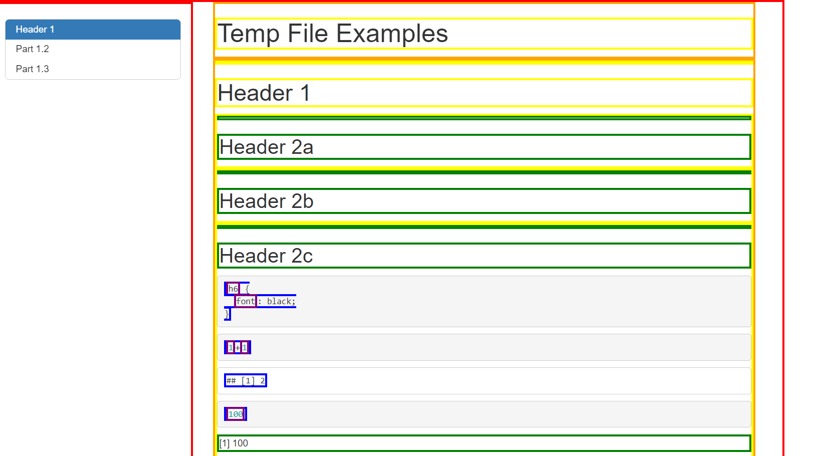
Experimentation: Finally, do not be afraid to experiment. It can sometimes be helpful to temporarily add style to items to help confirm or deny your understanding of the document structure. As a trivial example, the following CSS code draws brightly colored boxes around output at different levels of nesting. This could be useful to check visually review parent and child relationships between elements or notice invisible levels of nesting.

* * * * * { border: 3px solid red}
* * * * * * { border: 3px solid orange}
* * * * * * * { border: 3px solid yellow}
* * * * * * * * { border: 3px solid green}
* * * * * * * * * { border: 3px solid blue}
* * * * * * * * * * { border: 3px solid purple}
* * * * * * * * * * * { border: 3px solid pink}

Here’s an example of what applying this to a standard R Markdown output looks like:

Iterate faster with an external CSS file: By default, rmarkdown renders documents to a single file and embeds related assets such as CSS, JavaScript, and images. Having a standalone document is convenient for sharing your results, but this embedding makes it harder to quickly edit your CSS to test out different options. If you want to modify the CSS of a rendered self-contained R Markdown document, you must find the CSS code embedded in a large raw HTML file or render the whole document again (including running R code and Pandoc). To iterate more quickly, set the rmarkdown::html_document option to self_contained: false and use the css option to pass a file path to an external CSS file. Your resulting HTML document will contain a reference to this file on your computer. Thus, after rendering, you may continue to modify the CSS file in a text editor and see the changes to your HTML document without running any code again; you may simply refresh the web browser that you are using to view the document or close and reopen your file.

Footnotes

1. However, when the chunk option results = 'asis' is set, output is wrapped in <p> tags instead.